Waypoint Setting Via Webcam and OpenCV
ECE 439 Final Project - May 2020
Download the full project report here.
Abstract
Demo Video
Design
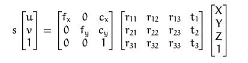
For the vision processing, we chose to use OpenCV due to its native integration with ROS. The OpenCV API also includes simple functions for performing perspective transformations that are required to gather 3D locations from our 2D webcam data. These functions are built on what is known as the pinhole camera model, which drastically simplifies the math required to do the transformation, without sacrificing significant accuracy. The model is shown below in Equation 1.
where:
- s is the scaling factor, used to scale the distance values to the camera
- [u, v, 1] is the homogeneous camera coordinates, or the point on the screen that is clicked
- fx and fy are the focal lengths of our camera lens
- cx and cy are the camera coordinates of the center of our image
- r and t represent the rotation and translation of our camera in the world frame
- [X, Y, Z, 1] is the homogeneous world coordinates of the point we clicked
The matrix consisting of f and c is also called the intrinsic or camera matrix. The matrix consisting of r and t is called the extrinsic matrix. Solving for the world coordinates is then just a matter of finding these matrices and solving the above equation for X, Y, and Z. Thankfully, OpenCV also has tools for us to generate these intrinsic (camera) and extrinsic matrices.
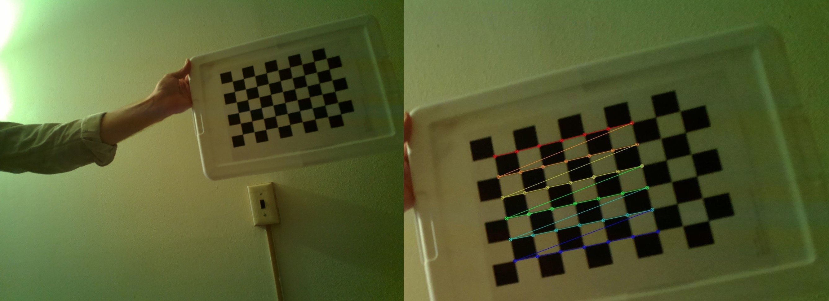
The first step was to find the camera matrix by measuring
distortions in our camera. In order to do this, we took 16 images of
a standard chessboard pattern. After gathering the images, we loaded
them into a python script provided by OpenCV, which identifies the
chessboard pattern and measures how much the straight chessboard
lines are distorted by the camera. Using OpenCV’s
calibrateCamera and
getOptimalNewCameraMatrix, we can then load the found
camera matrix into our runtime code.
We found that the Raspberry Pi did not have the required processing power to perform some of the computer vision algorithms necessary for the calibration. Because of this, the calibration step was completed using a Python script on a desktop computer.
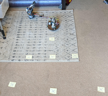
Next we had to generate the extrinsic matrix by perspective
calibration. This process involved placing marks on the ground at
known locations and gathering their (u, v) screen-space coordinates.
After gathering these points, we generated the extrinsic matrix with
OpenCV’s
solvePNP function.
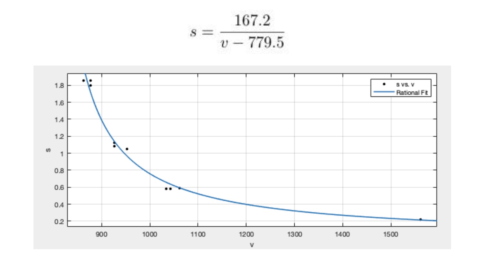
The last piece of information we needed was the scaling factor. Originally, we expected the scaling factor to be a single value dependent on the geometry of the transformation. The solvePNP function, however, gave a range of scaling values that appeared to have a positive correlation with the v-coordinate. Exploiting this observation, we were able to fit an equation to our perspective calibration data to find s in terms of the v-coordinate:
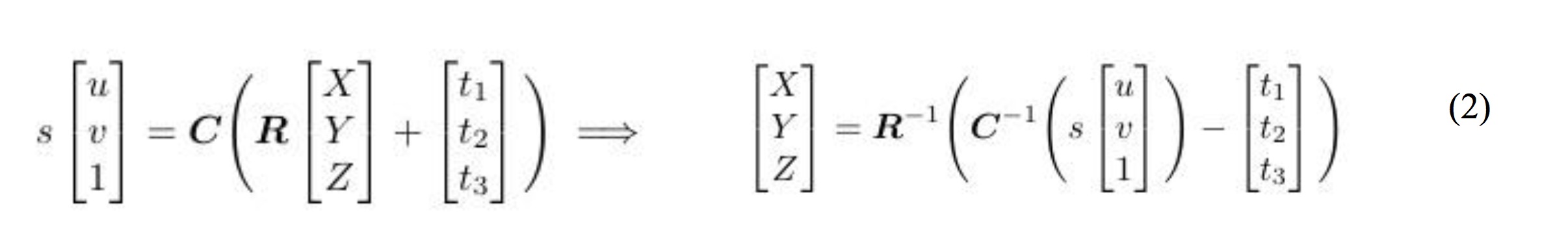
We then had all of the information needed to solve the 3D reconstruction equation. The intrinsic and extrinsic matrices were saved to the ROS working directory so that these calibrations did not have to be run each time the program was started. We then generated the 3D location by inverting our camera (C) and rotation (R) matrices and using them to solve for the world coordinates (Equation 2).
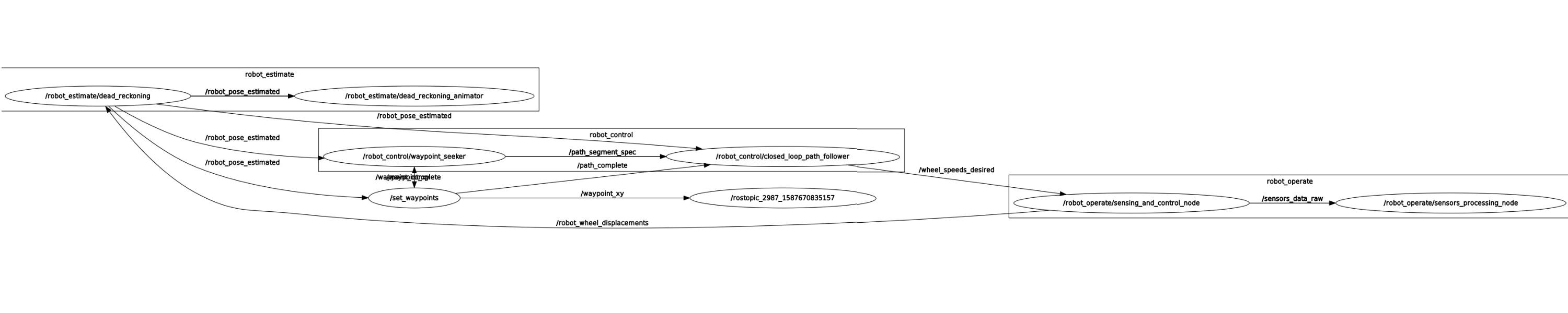
The last goal was then to implement this new waypoint information
into a ROS node. We modified the set_waypoints.py node
from class to incorporate our computer vision code. Since the camera
is mounted to the robot, the 3D reconstruction provides coordinates
in the robot’s coordinate frame. In order to convert this to a
waypoint, we transformed the coordinate in the robot’s frame back to
the world frame using the current position and heading of the robot:
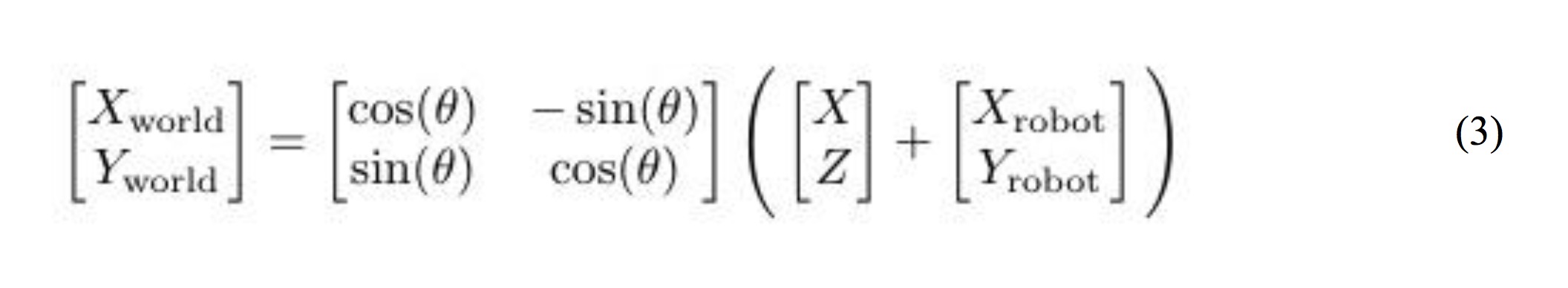
where X and Z are the 3D reconstructed points from above1, the robot coordinates are the 2D position of the robot, and theta is the robot’s pose angle relative to world “North”.
After transforming into the world coordinates, we simply published
our new waypoint to the waypoint_xy ROS topic and set
path_complete to be false so the
waypoint_follower knows to begin tracking a path to the
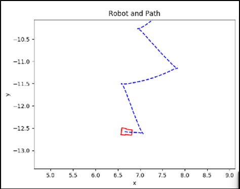
next waypoint. One unexpected difficulty we ran into while running
our code was the magnitude of the strain that processing the video
put on the CPU of the Raspberry Pi. Because of this, our robot would
often receive delayed control signals, causing it to go haywire not
long after starting the program (Figure 5). To cope with this, we
reduced the resolution of the video and scaled the (u,v) coordinates
accordingly, which allowed the robot to maintain stability while
running the program.
Another issue we ran into was that it was difficult to make sharp
turns and easily maneuver the robot due to the limited field of view
of the camera. To solve this, we attached the camera to a servo
which allowed us to turn the camera left and right to make sharper
turns. Our initial plan was to implement this in the
set_waypoints node, but we ran into some issues with
running multiple GUIs in one ROS node. Instead, we created a new
node which launches a servo control slider and sends the PWM signal
data to the waypoint setting node, and this seemed to work much
better. Once the waypoint setting node gets the PWM signal, the
camera rotation angle is known. The X and Z coordinates in Equation
3 are then rotated by this angle before determining the X and Y
world coordinates.
Footnotes:
1Note that the Z value from our 3D reconstruction is actually the Y value in our ROS waypoint code. The discrepancy is due to how OpenCV defines the coordinates of the pinhole camera model vs. the coordinate system we have used all semester
Results
To assess the performance of our new control method, we set up a series of targets at increasing distance from the robot. After moving to each target, the error was measured and recorded, and this can be seen in Figure 7. From this data, it is clear that the robot was the most accurate at distances of approximately 0.6 to 1.5 meters. At points closer than 0.6 meters and farther than 1.5 meters, the error starts to increase greatly. This error is to be expected due to the camera’s proximity to the ground. Far distances are compressed into a very small v-coordinate range, so clicking them accurately is difficult. The far-distance error could be improved by raising the camera, but this was not practical for our small mobile robot.
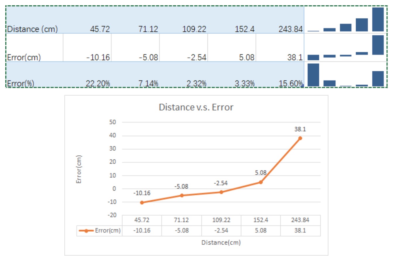
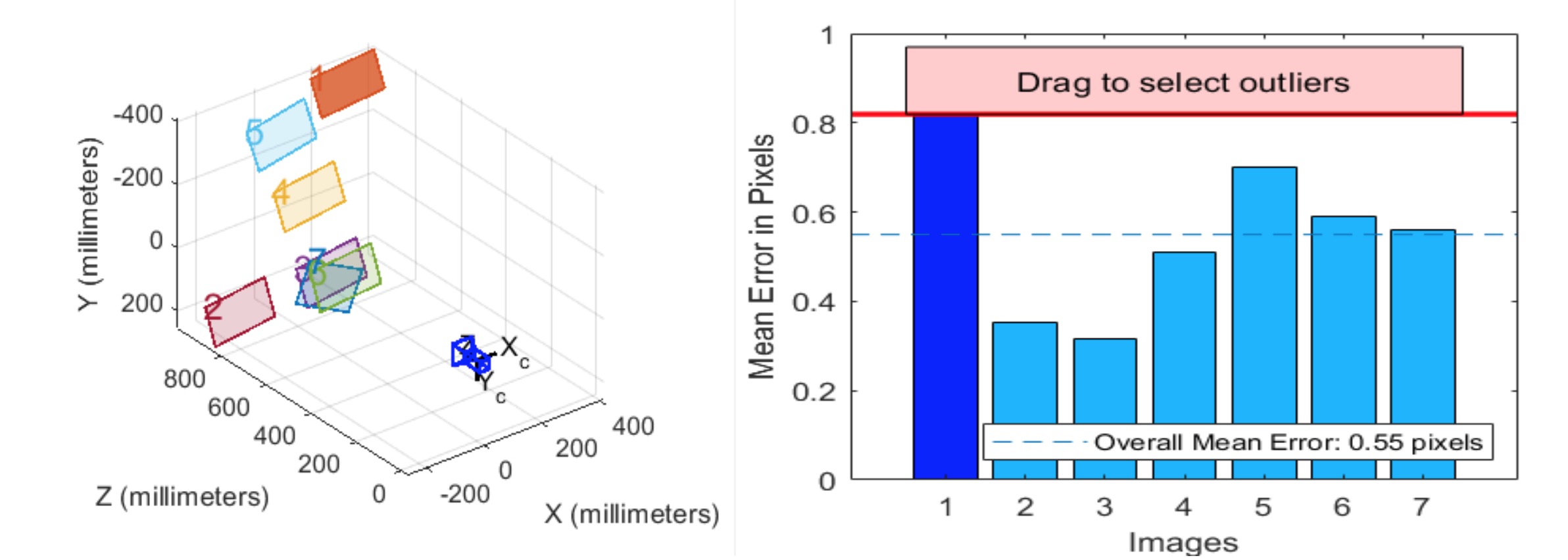
The short-distance error could potentially be due to our intrinsic camera calibration. Closer objects are more heavily affected by camera distortion, so if the calibration is not perfect, these waypoints could be transformed incorrectly. We took several chessboard images and only used the best seven images in order to get the calibration results with least error. Ideally, we would have used more images in our calibration. As long as the user specifies waypoints within two meters of the robot, error values are well-controlled.
We tested maneuvering the robot through an apartment without line-of-sight, and it is simple to spot obstacles in the webcam and use the OpenCV interface to avoid them. Important challenges included maneuvering around blind corners by rotating the webcam, and adjusting the path on-the-fly as new obstacles are spotted. After multiple successful runs, we conclude that our concept of gathering waypoint from a webcam image is a successful method of teleoperated robot control.
Discussion
The robot was able to move to the position with relatively high precision (error within 10%) if the distance to the target is within the range of 0.6 meters to 1.5 meters. We may be seeing this improved accuracy because this is the range which we used to calibrate our camera. As we try setting waypoints farther from the robot, the trigonometry that is used to solve for the world coordinates starts approaching a vertical asymptote. This may be what is contributing to the larger errors that we see in these locations. Those errors could possibly come from the intrinsic matrix that we get from the initial calibration, extrinsic matrix and the scaling factor from the perspective calibration. Moreover, we couldn’t undistort the video due to the processing speed of Raspberry Pi, as it is relayed to the user, so the distorted image clicked by the user could cause few-pixel inaccuracy, and that could result in higher error for points at the edge of the images.
All in all, this project taught us quite a bit about some basic things that can be done with OpenCV and how to incorporate a project idea into a working ROS infrastructure. We were successfully able to undistort our camera image and perform a perspective calibration using OpenCV’s camera calibration functions, which also taught us quite a bit on the intrinsic parameters of a camera and how to use two-dimensional camera coordinates to predict three-dimensional coordinates in a world frame. We were also able to adjust our waypoint setting node to consistently take in and hold one set of coordinates at a time. Setting up this communication between ROS and OpenCV proved to be one of our most challenging goals.
There are many future goals that we would have liked to implement given more time. For instance, our current workflow does not handle invalid data points very well. Clicks above or near the horizon will either result in y-coordinates that are negative or extremely large, and the extent of this can be seen by our increasing error with increasing target y-values. A limit could be placed either on y-coordinate or v-coordinate values to prevent such errors. We would have also liked to integrate some form of obstacle avoidance, or at the very least obstacle detection, to deal with path entries that pass through obstacles or enter bounded areas, such as the opposite sides of walls. Hand-in-hand with this would be the addition of a SLAM algorithm. It would be interesting to have a mapped augmented reality environment which would allow the user to select locations in other areas of the map that the robot can’t see with the camera. The robot could then use the map to plan a path to this location accordingly. These are just a few examples of the many ways in which the usability of this control mechanism could be improved.
References
"Calculate X, Y, Z Real World Coordinates from Image ...." 10 Apr. 2019, https://www.fdxlabs.com/calculate-x-y-z-real-world-coordinates-from-a-single-camera-using-opencv/. Accessed 4 May. 2020.
"Camera Calibration - OpenCV-Python Tutorials - Read the Docs." http://opencv-python-tutroals.readthedocs.io/en/latest/py_tutorials/py_calib3d/py_calibration/py_calibration.html. Accessed 4 May. 2020.
"Camera Calibration and 3D Reconstruction — OpenCV 2.4 ...." 31 Dec. 2019, https://docs.opencv.org/2.4/modules/calib3d/doc/camera_calibration_and_3d_reconstruction.html. Accessed 4 May. 2020.
Canu, S. "Mouse Events – OpenCV 3.4 with python 3 Tutorial ... - Pysource." 27 Mar. 2018, https://pysource.com/2018/03/27/mouse-events-opencv-3-4-with-python-3-tutorial-27/. Accessed 4 May. 2020.